Getting started

The iucm package uses the model-organization framework and thus can be used from the command line. The corresponding subclass of the model_organization.ModelOrganizer is the iucm.main.IUCMOrganizer class.

In this section, we provide a small starter example that transforms a fictitious city by moving 125‘000 inhabitants. Additional to the already mentioned requirements, this tutorial needs the psy-simple plugin and the pyshp package.

After having installed the package you can setup a new project with the iucm setup command via

In [1]: !iucm setup . -p my_first_project
INFO:iucm.my_first_project:Initializing project my_first_project

To create a new experiment inside the project, use the iucm init command:

In [2]: !iucm -id my_first_experiment init -p my_first_project
INFO:iucm.my_first_experiment:Initializing experiment my_first_experiment of project my_first_project

Running the model, only requires a netCDF file with absolute population data. The x-coordinates and y-coordinates must be in metres.

Transforming a city

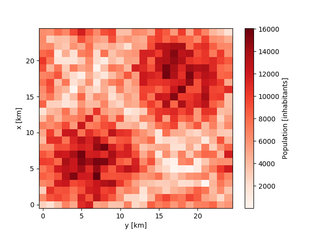
For the purpose of demonstration, we simply create a random input file with 2 city centers on a 25km x 25km grid at a resolution of 1km.

In [3]: import numpy as np
   ...: import xarray as xr
   ...: import matplotlib.pyplot as plt
   ...: import psyplot.project as psy
   ...: np.random.seed(1234)
   ...: 

In [4]: sine_vals = np.sin(np.linspace(0, 2 * np.pi, 25)) * 5000
   ...: x2d, y2d = np.meshgrid(sine_vals, sine_vals)
   ...: data = np.abs(x2d + y2d) + np.random.randint(0, 7000, (25, 25))
   ...: 

In [5]: population = xr.DataArray(
   ...:     data,
   ...:     name='population',
   ...:     dims=('x', 'y'),
   ...:     coords={'x': xr.Variable(('x', ), np.arange(25, dtype=float),
   ...:                              attrs={'units': 'km'}),
   ...:             'y': xr.Variable(('y', ), np.arange(25, dtype=float),
   ...:                              attrs={'units': 'km'})},
   ...:     attrs={'units': 'inhabitants', 'long_name': 'Population'})
   ...: 

In [6]: population.plot.pcolormesh(cmap='Reds');

In [7]: population.to_netcdf('input.nc')

Now we create a new scenario where we transform the city by moving stepwise 500 inhabitants around. For this, we need a forcing file which we can create using the iucm preproc forcing command:

In [8]: !iucm -v preproc forcing -steps 50 -trans 500
INFO:iucm.my_first_experiment:Creating forcing data...
DEBUG:iucm.my_first_experiment:Saving output to /home/docs/checkouts/readthedocs.org/user_builds/iucm/checkouts/latest/docs/my_first_project/experiments/my_first_experiment/input/forcing.nc
DEBUG:iucm.my_first_experiment:    development_file: None
DEBUG:iucm.my_first_experiment:    development_steps: [100]
DEBUG:iucm.my_first_experiment:    trans_size: 500.0
DEBUG:iucm.my_first_experiment:    total_steps: 100
DEBUG:iucm.my_first_experiment:    movement: 0

This now did create a new netCDF file with two variables

In [9]: xr.open_dataset(
   ...:     'my_first_project/experiments/my_first_experiment/input/forcing.nc')
   ...: 
Out[9]: 
<xarray.Dataset>
Dimensions:   (step: 100)
Coordinates:
  * step      (step) int64 1 2 3 4 5 6 7 8 9 10 ... 92 93 94 95 96 97 98 99 100
Data variables:
    change    (step) float64 ...
    movement  (step) int64 ...

that is also registered as forcing file in the experiment configuration

In [10]: !iucm info -nf
id: my_first_experiment
project: my_first_project
expdir: experiments/my_first_experiment
timestamps:
  init: '2018-12-28 22:59:55.010261'
  setup: '2018-12-28 22:59:53.270020'
  preproc: '2018-12-28 22:59:57.633896'
indir: experiments/my_first_experiment/input
preproc:
  forcing:
    development_file: null
    development_steps:
    - 100
    trans_size: 500.0
    total_steps: 100
    movement: 0
forcing: experiments/my_first_experiment/input/forcing.nc

The change variable in this forcing file describes the number of people that are moving within each step. In our case, this is just an alternating series of 500 and -500 since we take 500 inhabitants from one grid cell and move it to another.

Having prepared this input file, we can run our experiment with the iucm run command:

In [11]: !iucm -id my_first_experiment configure -s run -i input.nc -t 50 -max 15000
INFO:iucm.model:Saving to /home/docs/checkouts/readthedocs.org/user_builds/iucm/checkouts/latest/docs/my_first_project/experiments/my_first_experiment/outdata/my_first_experiment_1-50.nc...

The options here in detail:

-id my_first_experiment

Tells iucm the experiment to use. The -id option is optional. If omitted, iucm uses the last created experiment.

configure -s

This subcommand modifies the configuration to run our model in serial (see iucm configure)

run

The iucm run command which tells iucm to run the experiment. The options here are

-t 50

Tells to model to make 50 steps

-max 15000

Tells the model that the maximum population is 15000 inhabitants per grid cell

The output now is a netCDF file with 50 steps:

In [12]: ds = xr.open_dataset(
   ....:     'my_first_project/experiments/my_first_experiment/'
   ....:     'outdata/my_first_experiment_1-50.nc')
   ....: 

In [13]: ds
Out[13]: 
<xarray.Dataset>
Dimensions:        (en_variables: 5, probabilistic: 1, step: 50, x: 25, y: 25)
Coordinates:
  * x              (x) float64 0.0 1.0 2.0 3.0 4.0 ... 20.0 21.0 22.0 23.0 24.0
  * y              (y) float64 0.0 1.0 2.0 3.0 4.0 ... 20.0 21.0 22.0 23.0 24.0
  * step           (step) int64 1 2 3 4 5 6 7 8 9 ... 42 43 44 45 46 47 48 49 50
  * en_variables   (en_variables) object 'k' 'dist' 'entrop' 'rss' 'own'
Dimensions without coordinates: probabilistic
Data variables:
    population     (step, x, y) float64 ...
    cons           (step) float64 ...
    dist           (step) float64 ...
    entrop         (step) float64 ...
    rss            (step) float64 ...
    cons_det       (step) float64 ...
    cons_std       (step) float64 ...
    left_over      (step) float64 ...
    nscenarios     (step) float64 ...
    cons_2d        (step, x, y) float64 ...
    dist_2d        (step, x, y) float64 ...
    entrop_2d      (step, x, y) float64 ...
    rss_2d         (step, x, y) float64 ...
    cons_det_2d    (step, x, y) float64 ...
    cons_std_2d    (step, x, y) float64 ...
    left_over_2d   (step, x, y) float64 ...
    nscenarios_2d  (step, x, y) float64 ...
    scenarios_2d   (step, x, y) float64 ...
    weights        (step, en_variables, probabilistic) float64 ...

With the output for the population, energy consumption and other variables. In the last step we also see, that the new population has mainly be added to the city centers in order to minimize the transportation energy:

In [14]: fig = plt.figure(figsize=(14, 6))
   ....: fig.subplots_adjust(hspace=0.5)
   ....: 

# plot the energy consumption
In [15]: ds.cons.psy.plot.lineplot(
   ....:     ax=plt.subplot2grid((4, 2), (0, 0), 1, 2),
   ....:     ylabel='{desc}', xlabel='%(name)s');
   ....: 

In [16]: ds.population[-1].psy.plot.plot2d(
   ....:     ax=plt.subplot2grid((4, 2), (1, 0), 3, 1),
   ....:     cmap='Reds', clabel='Population');
   ....: 

In [17]: (ds.population[-1] - population).psy.plot.plot2d(
   ....:     ax=plt.subplot2grid((4, 2), (1, 1), 3, 1),
   ....:     bounds='roundedsym', cmap='RdBu_r',
   ....:     clabel='Population difference');
   ....: 

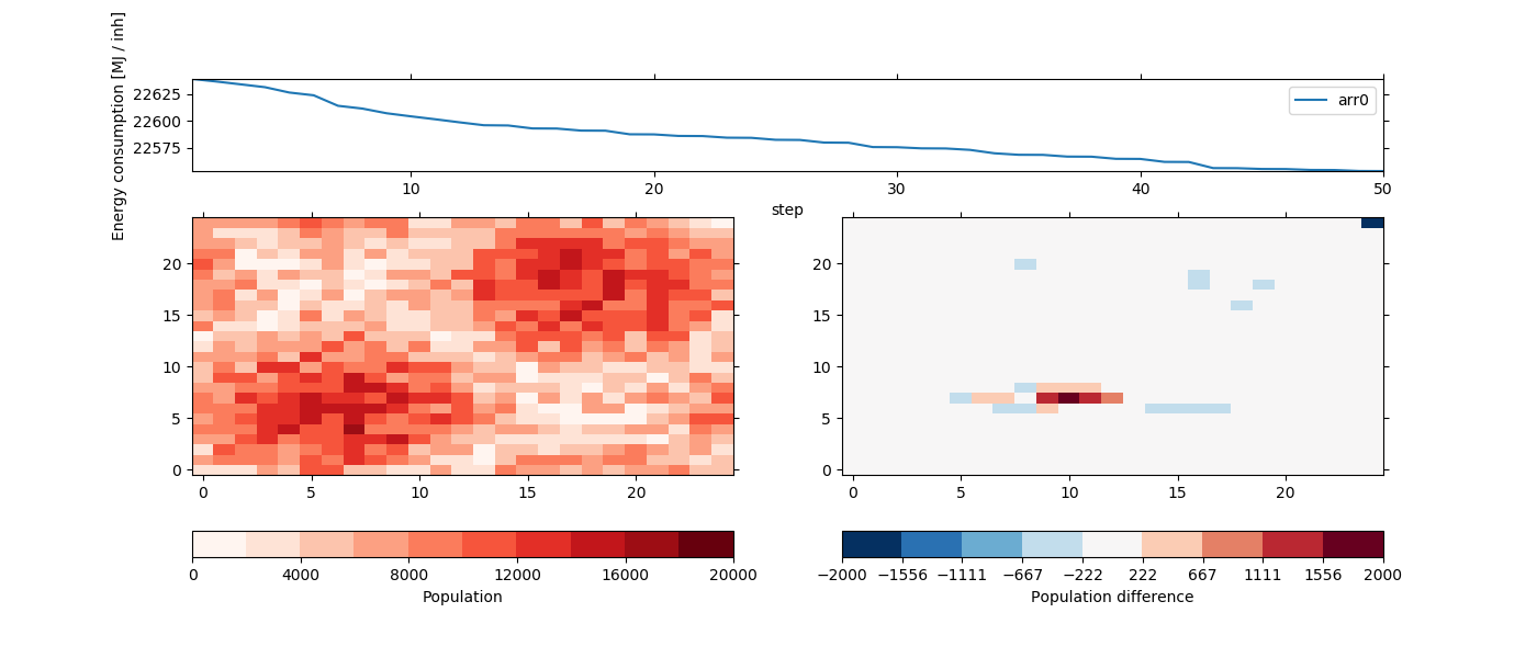
As we can see, the model did move the population of sparse cells to locations where the population is higher, mainly to decrease the average distance between two individuals within the city.

The run settings are now stored in the configuration of the experiment, which can be seen via the iucm info command:

In [18]: !iucm info -nf
id: my_first_experiment
project: my_first_project
expdir: experiments/my_first_experiment
timestamps:
  init: '2018-12-28 22:59:55.010261'
  setup: '2018-12-28 22:59:53.270020'
  preproc: '2018-12-28 22:59:57.633896'
  run: '2018-12-28 23:00:11.258889'
  configure: '2018-12-28 23:00:01.185258'
indir: experiments/my_first_experiment/input
preproc:
  forcing:
    development_file: null
    development_steps:
    - 100
    trans_size: 500.0
    total_steps: 100
    movement: 0
forcing: experiments/my_first_experiment/input/forcing.nc
run:
  ncells: 4
  selection_method: consecutive
  update_method: forced
  categories:
  - null
  - 15000.0
  probabilistic: 0
  max_pop: 15000.0
  coord_transform: 1.0
  steps: 50
  step_date:
    50: '2018-12-28 23:00:01.675781'
  vname: population
outdir: experiments/my_first_experiment/outdata
outdata:
- experiments/my_first_experiment/outdata/my_first_experiment_1-50.nc
input: experiments/my_first_experiment/input/input.nc

Probabilistic model

The default IUCM settings use a purely deterministic methodology based on the regression by [LeNechet2012]. However, to take the errors of this model into account, there exists a probabilistic version that is simply enabled via the -prob (or --probabilistic) argument, e.g. via

In [19]: !iucm run -nr -prob 1000 -t 50
INFO:iucm.model:Saving to /home/docs/checkouts/readthedocs.org/user_builds/iucm/checkouts/latest/docs/my_first_project/experiments/my_first_experiment/outdata/my_first_experiment_1-50.nc...

Instead of simply moving population from one cell to another, it distributes the population to multiple cells based on their probability to lower the energy consumption for the city.

In [20]: ds = xr.open_dataset(
   ....:     'my_first_project/experiments/my_first_experiment/'
   ....:     'outdata/my_first_experiment_1-50.nc')
   ....: 

In [21]: plot_result()

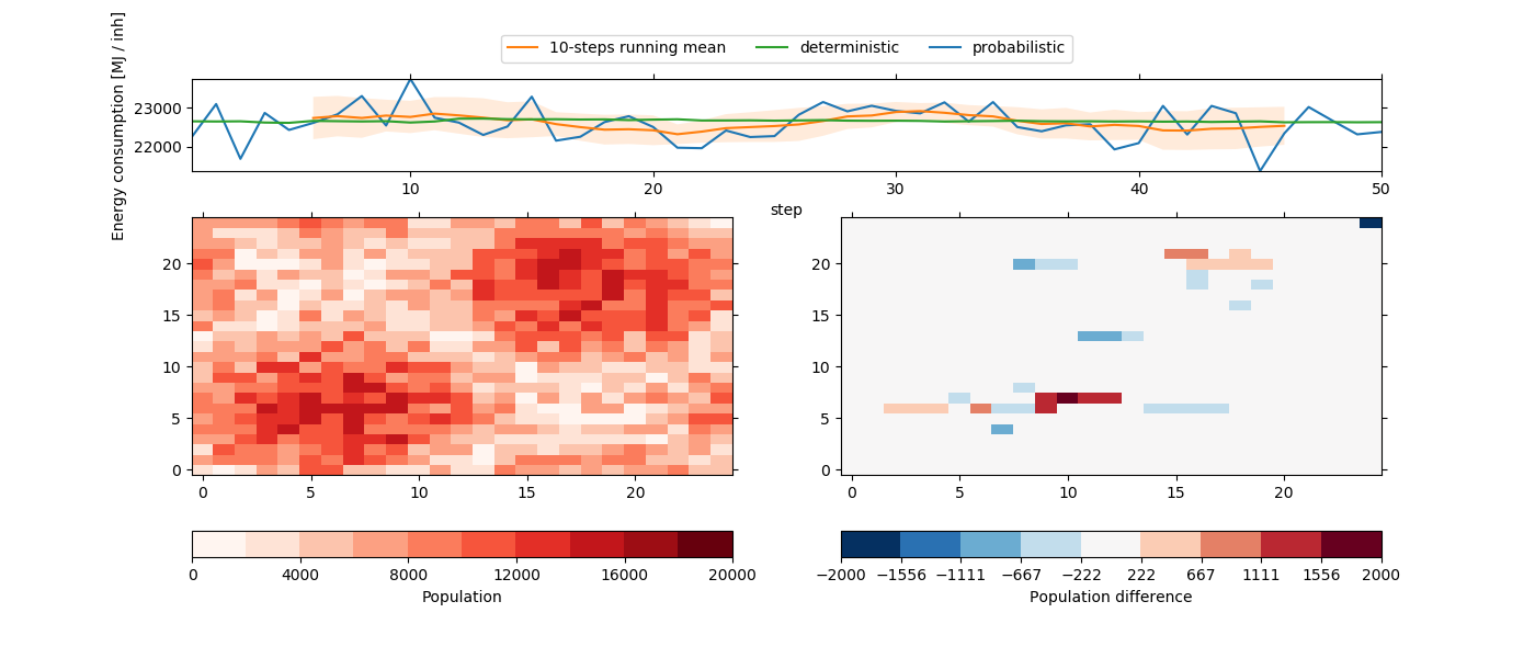
As we can see, the results are not as smooth as the deterministic results, because now the energy consumption is based on a probabilistic set of regression weights (see iucm.energy_consumption.random_weights()). On the other hand, the deterministic energy consumption (stored as variable cons_det in the output file) corresponds pretty much to the deterministic version of our experiment setup above, as well as the running mean. And indeed, if we would drastically increase the number of probabilistic scenarios, we would approximate this energy consumption curve.

Note

The energy consumption in the output file is for the probabilistic setting determined by the mean energy consumption for all random scenarios. The cons_det variable on the other hand is always determined by the weights in [LeNechet2012] (see iucm.energy_consumption.weights_LeNechet)

Masking areas

Each city has several areas that should not be filled with population, such as rivers, parks, etc. For example we assume a river, a lake and a forest in our city (see the zipped shapefile)

In [22]: population.plot.pcolormesh(cmap='Reds');

In [23]: from shapefile import Reader
   ....: reader = Reader('masking_shapes.shp')
   ....: 

In [24]: from matplotlib.patches import Polygon
   ....: ax = plt.gca()
   ....: for shape_rec in reader.iterShapeRecords():
   ....:     color = 'forestgreen' if shape_rec.record[0] == 'Forest' else 'aqua'
   ....:     poly = Polygon(shape_rec.shape.points, facecolor=color, alpha=0.75)
   ....:     ax.add_patch(poly)
   ....: 

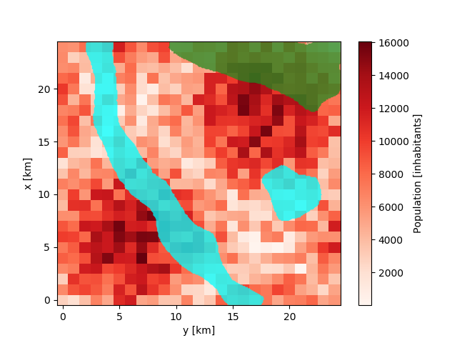
IUCM has three options, how to handle these areas:

ignore

The cells and the population that are touched by these shapes are completely ignored

mask

The cells are masked for keeping their population constant

max-pop

The maximum population in the cells that are touched by the shapes is lowered by the fraction that the shape cover in each cell

All three methods can easily be applied using the iucm preproc mask command.

Note

Using this feature requires pyshp to be installed and the shapefile must be defined on the same coordinate system as the input data!

Ignoring the areas

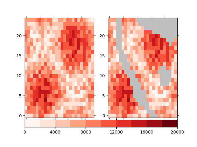
Ignoring the shapes will set the grid cells that are touched by the given shapefiles to NaN, i.e. not a number. Input cells that contain this value are completely ignored in the simulation. For our shapefile and input data here, the result would look like

In [25]: fig, axes = plt.subplots(1, 2)

In [26]: plotter = population.psy.plot.plot2d(
   ....:     ax=axes[0], cmap='Reds', cbar='')
   ....: 

In [27]: !iucm preproc mask masking_shapes.shp -m ignore

In [28]: sp = psy.plot.plot2d('input.nc', name='population', ax=axes[1],
   ....:                      cmap='Reds', cbar='fb', miss_color='0.75')
   ....: sp.share(plotter, keys='bounds')
   ....: 

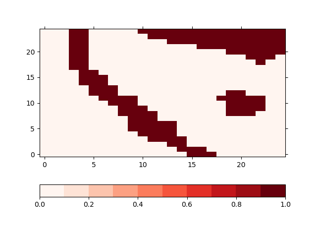
Masking the areas

Masking the areas means, that the population data in the grid cells that touch the given cells is not changed but it is considered in the calculation of the energy consumption. The input file for the model has a designated variable named mask for that. The population data for non-zero grid cells in this variable will be kept constant. In our case, the resulting mask variable in looks like this

In [29]: !iucm preproc mask masking_shapes.shp -m mask

In [30]: sp = psy.plot.plot2d('input.nc', name='mask', cmap='Reds')

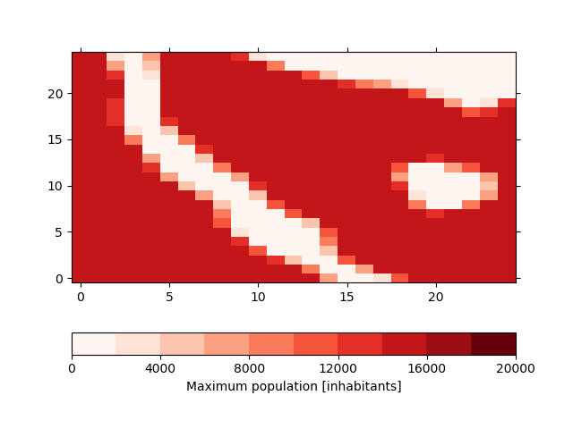
Adjusting the maximum population

This is the default method and is the best method represent the shape files in the model. Instead of masking the data, we lower the amount of the maximum possible population in the grid cells. For this, the shapefile is rasterized at high resolution (by default 100-times the resolution of the input file) and the we calculate the percentage for each coarse grid cell that is covered by the shape. The result will then be stored in the max_pop variable in the input dataset which defines the maximum population for each grid cell. In our case, this variable looks like

In [31]: !iucm preproc mask masking_shapes.shp

In [32]: sp = psy.plot.plot2d('input.nc', name='max_pop', cmap='Reds',
   ....:                      clabel='{desc}')
   ....: 

Note

This method is a pure python implementation that does not have any other dependencies than matplotlib and pyshp. Due to this, it might be slow for large shapefiles or large input files. In this case, we recommend to use gdal_rasterize for creating the high resolution rastered shape file and gdalwarp for interpolating it to the input grid. In our case here, this would look like

gdal_rasterize -burn 1.0 -tr 0.01 0.01 masking_shapes.shp hr_rastered_shapes.tif
gdalwarp -tr 1.0 1.0 -r average hr_rastered_shapes.tif covered_fraction.tif
gdal_calc.py -A covered_fraction.tif --outfile=max_pop.nc --format=netCDF --calc="(1-A)*15000"

And then merge the file 'max_pop.nc' into 'input.nc' as variable 'max_pop'.